Greenhouses provide growers with a way to manage the growing environment more effectively than open fields. However, finding the right balance between all the variables—like temperature, humidity, and CO2 concentration—is tricky. There are so many factors at play, and sometimes they even conflict with one another! That’s why it’s so important to use optimal diurnal climate control to boost crop quality, yield, and profitability.
In this guide, we’ll break down different techniques for controlling your greenhouse’s climate to meet your crop’s specific needs. Let’s get into how you can make the most of modern greenhouse tech.
Section 1: What is Optimal Climate Control?
In simple terms, optimal climate control means creating the best possible environment for your crops based on your goals. Whether you’re focused on maximizing yield, reducing costs, or improving crop quality, climate control is key. The challenge lies in balancing all these factors—because what’s good for yield might not always be great for quality. So, how do we strike that balance?
Section 2: Different Levels of Greenhouse Management
Greenhouse management can be broken down into three levels: strategical, tactical, and operational.
- Strategical Management: This is your long-term planning—deciding what equipment to invest in or what type of greenhouse to build. It’s all about setting yourself up for success years down the road.
- Tactical Management: Once you’ve got your big plans in place, you need to decide what crops to grow and when to plant them. This includes setting up a plan for how you’ll control the climate during the growing season.
- Operational Management: Here’s where you handle the day-to-day adjustments. Maybe the weather didn’t go as planned, or your crop is growing differently than expected. At this level, you’re tweaking the climate to keep things on track.
Section 3: Criteria for Climate Control in Greenhouses
To achieve optimal control, you need to consider several factors that directly affect your crops:
- Physical Yield: Yield is heavily influenced by climate conditions, particularly light and CO2 levels. But keep in mind that increasing yield too quickly could affect long-term crop health.
- Crop Quality: Keeping crops in good condition for the long haul is crucial, especially with long-growing plants. Temperature control plays a significant role here, helping you maintain the right balance between vegetative and generative growth.
- Product Quality: This is all about the final look and taste of your crops. How big are they? What’s their shape and color? Temperature and humidity are major players here, but the connection between climate and product quality can be tricky to pin down.
- Timing: Whether you’re aiming to hit seasonal markets (think Christmas poinsettias) or just need efficient space utilization, timing is key. You can control this with temperature and light adjustments.
- Cost Management: Running a greenhouse isn’t cheap, especially when you factor in the costs of heating, CO2 enrichment, and extra lighting. Careful climate control can help reduce some of these expenses.
- Risk Prevention: Greenhouses offer a level of protection against pests, diseases, and environmental stress. Controlling humidity and temperature within certain limits helps keep your plants safe and reduces the need for pesticides.
Section 4: Key Techniques for Diurnal Climate Control
Let’s get into the actual tools you can use to manage your greenhouse climate:
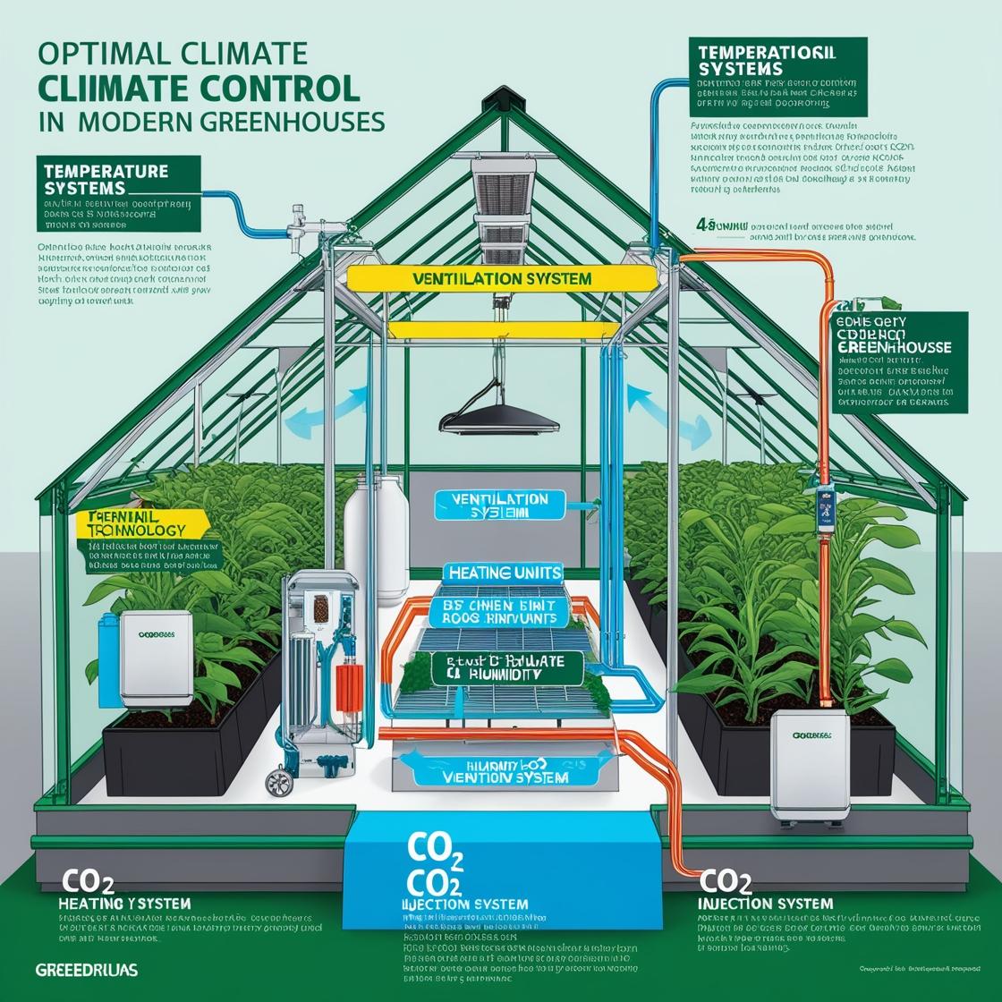
- Ventilation and Heating: You can control both temperature and humidity with the right combination of ventilation and heating systems. This is essential to keep your crops growing in the ideal conditions.
- CO2 Enrichment: Want to boost photosynthesis and increase your yield? CO2 enrichment is the way to go. It can be done through flue gases or pure CO2 sources.
- Lighting and Screens: Screens and supplemental lighting help you adjust radiation levels inside the greenhouse, especially during shorter days or low-light conditions.
- Soilless Culture: For those using hydroponics or other soilless methods, it’s easier to control the nutrient and water levels, which can be quickly adjusted based on the crop’s needs.
Actionable Tips for Growers
- Invest in quality climate control systems: Prioritize tools that allow you to adjust ventilation, heating, and lighting. The more control you have, the better.
- Track crop performance regularly: Don’t just set your climate controls and forget them. Keep an eye on your crops and adjust as needed to ensure they’re growing in the best conditions.
- Be proactive with CO2 enrichment: If your goal is to maximize yield, make sure to implement CO2 enrichment in your greenhouse. It’s a game-changer for increasing photosynthesis.
- Balance short-term and long-term goals: Pushing for a quick yield increase can lead to crop health problems down the road. Always consider how today’s decisions will impact tomorrow’s results.
Conclusion
Optimal diurnal climate control in greenhouses isn’t just about managing temperature—it’s a balance between yield, crop quality, cost, and timing. To truly optimize your greenhouse, you need to manage these factors in harmony. And with modern technology, the tools to achieve this balance are right at your fingertips.
Summary for Instagram Reels/Infographics:
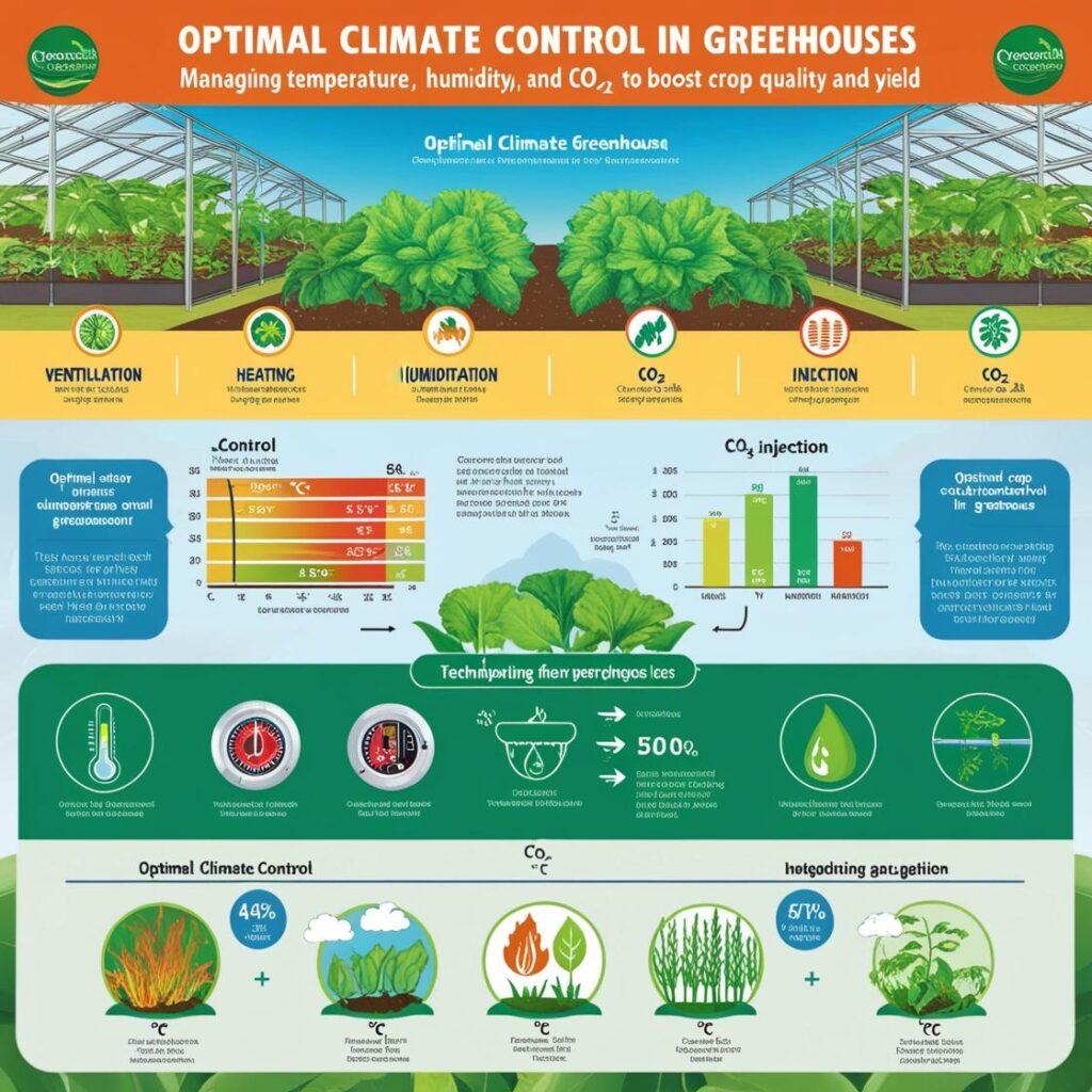
- Optimal Climate Control: Balancing temperature, humidity, and CO2 to meet crop goals.
- 3 Management Levels: Strategical (long-term), Tactical (crop-specific), Operational (day-to-day tweaks).
- Key Factors: Yield, crop quality, product quality, timing, cost, and risk prevention.
- Pro Tips: Invest in tech, track crop health, use CO2 enrichment, and balance short-term vs. long-term goals.
With these insights, you can easily create engaging content to share with your audience!
This text discusses the complex processes involved in greenhouse crop production and how they can be optimized through climate control.
1. Production Process: The crop production process begins with the trapping of solar energy, which is transformed into chemical energy used to reduce CO2 molecules. This energy is then utilized to create sugars and other organic compounds needed for growth. These building blocks are transported throughout the plant, supporting the development of cells and organs. The production process includes leaf formation, shoot development, and transitions between vegetative and generative phases. In relation to climate control, it is essential to classify crop reactions based on response type and time.
2. Response Types: Some crop reactions are smooth and continuous, while others have non-linear thresholds. Smooth reactions should always be considered in climate control, while threshold reactions are significant only when boundary conditions are exceeded. Managing these two types of responses simplifies climate control by focusing on continuous responses and respecting boundary conditions.
3. Response Time: The processes have different response times. Processes with slow response times (>24 hours) allow for more flexibility in controlling climate conditions. Short-term processes (<24 hours), such as photosynthesis, transpiration, and stress reactions, require immediate action and cannot be compensated later. Examples of short response processes include acute stress from temperature extremes, radiation, and water conditions.
4. Optimal Climate Control: Optimal control is part of overall management, and it requires ongoing adjustment to both short-term (minute-by-minute) and long-term (days to weeks) processes. Automatic climate control systems should optimize greenhouse conditions based on crop needs, market predictions, weather forecasts, and other data. Ideally, climate control is adjusted in real-time, with minimal grower interaction.
5. Economic Optimization: The goal of climate control is to maximize crop yield while minimizing associated costs, such as energy for heating and CO2 enrichment. The control system must balance economic returns from photosynthesis against operational costs. For generative crops like tomatoes, both costs and benefits are calculated continuously, while for vegetative crops like lettuce, economic yield is determined at the end of the growing season.
6. Model-Based Solutions: Mathematical models are used to simulate greenhouse and crop dynamics, helping to predict how climate control actions will affect plant growth. These models can be optimized to generate ideal climate control strategies over a set period. Advanced techniques, such as Hamiltonian methods, are used to calculate optimal control paths that maximize crop yield under given weather conditions and operational constraints.
7. Practical Considerations: Direct implementation of these solutions in real-world greenhouses is challenging due to weather unpredictability. Practical solutions include assigning economic value to photosynthesis, using feedback systems based on seasonal optimization, or employing neural networks to quickly compute control actions based on current conditions. These systems would need to be continuously updated as the actual process deviates from predictions.
8. Grower Interaction and Decision Support: Even with advanced climate control systems, grower input is crucial. The system should allow growers to set constraints and priorities, such as adjusting for weather changes or economic goals. The system must also be able to explain its decisions, providing confidence to growers.
In conclusion, effective climate control in greenhouses requires a combination of long-term optimization and real-time adjustments. The system must balance photosynthesis maximization with cost minimization, handle both slow and fast crop responses, and incorporate grower input for optimal decision-making.
IV. CONCLUSION
The optimal control of plant production in greenhouses involves addressing multiple, often conflicting goals, such as maximizing plant growth while minimizing energy consumption and pollution. Achieving this requires sophisticated control algorithms that integrate knowledge of plant physiology, environmental factors, and market conditions. A hierarchical and modular system, with different control levels for long-term planning, operational management, and real-time environmental control, allows for better management and optimization of resources. As more advanced models and data become available, techniques like feedback control, expert systems, and numerical optimization can improve decision-making and control in greenhouse environments.
By integrating plant growth models with environmental and economic data, growers can better plan for optimal production conditions, adjust to unexpected changes in climate or market, and ultimately achieve higher yields and profits while reducing their environmental footprint. Advanced technologies such as artificial intelligence, expert systems, and on-line optimization are essential for making greenhouse operations more efficient, flexible, and sustainable.
The development of more accurate plant models, alongside better control and monitoring systems, will allow for even finer control over the greenhouse environment. This includes real-time adjustments based on plant feedback and environmental changes. As greenhouse technology continues to evolve, it offers significant potential to not only increase productivity but also reduce resource use and environmental impact.
IV. ENVIRONMENTAL CONTROL (Bottom level)
In the realm of environmental control, significant research has focused on enhancing precision and efficiency at the bottom level of greenhouse operations. Modern greenhouses employ commercial climate control computers and substrate systems to manage water and nutrition supply effectively (Takakura, 1989). Despite these advancements, controlling greenhouse environments poses complex challenges from an engineering perspective, due to factors like system delays and long time constants (Veerwaaijen et al., 1985).
Greenhouse climate control is difficult because disturbances—such as changes in solar radiation, outdoor temperature, and wind velocity—rapidly affect internal conditions. Additionally, energy-saving methods like thermal screens can drastically reduce heat load in minutes, adding complexity to the control process.
To enhance control accuracy, adaptive control algorithms have been widely explored (Henten, 1989; Hooper, 1985; Tantau, 1985). Standard control methods such as proportional-integral-derivative (PID) controllers, commonly used in industrial processes, face limitations in greenhouses due to issues like inaccurate parameter estimation and unsatisfactory control behavior during the adaptive phase.
To overcome these challenges, modern greenhouses often combine feedback control with feedforward control. In this setup (as shown in Fig. 5), disturbance variables such as outdoor climate are measured, and actuators for heating, ventilation, shading, lighting, CO₂, and irrigation respond based on process models. Feedback control ensures stability and accuracy, while feedforward control allows for anticipatory adjustments to prevent overshoots or undershoots in temperature or humidity


Feedforward control has several advantages:
- Improved control loop stability.
- Early response to outdoor weather changes.
- Prevention of large actuator movements and overshooting.
- Reduced energy consumption through precise climate management.
However, feedforward control also requires on-line process identification and model parameter adaptation, which presents challenges like inaccurate parameter estimation and model “bursting.” Statistical methods and optimization techniques are employed to address these issues and fine-tune control parameters for real-time applications.
V. CONCLUSIONS
Research into greenhouse environmental control has primarily focused on the bottom level, yielding substantial improvements in control precision, system stability, and energy efficiency. These advances form the foundation for optimizing plant production at the middle level. However, a significant challenge remains in incorporating plant response models into real-time control systems. The lack of comprehensive knowledge about plant-environment interactions limits the application of online optimization in commercial greenhouses.
Expert systems offer a promising approach to integrate heuristic knowledge into control systems, potentially providing a user-friendly interface for growers. Further research is needed to develop “explanation units” that can handle uncertainty and enhance system reliability. Additionally, standardizing communication between different levels of control (especially between the top and middle levels) is crucial for future advancements in greenhouse optimization.
OPTIMAL GREENHOUSE TEMPERATURE TRAJECTORIES FOR A MULTI-STATE-VARIABLE TOMATO MODEL
In the study of optimal greenhouse temperature control, especially for crops like tomatoes, it is essential to balance various biological processes, particularly photosynthesis and development. While increasing photosynthesis is usually desirable, certain situations may require slowing plant development to meet specific production timelines. These conflicting objectives necessitate a sophisticated approach to control temperature in greenhouses.
The ideal solution involves using advanced control techniques such as the Pontryagin Maximum Principle (PMP) or dynamic programming. However, these methods require extensive computational resources, making them impractical for real-time control in multi-variable crop models. Instead, researchers have explored alternative methods like Sequential Control Search (SCS), which simplifies the process by focusing on short-term optimization decisions.
Studies show that SCS, though a simpler approach, yields results comparable to more complex methods like PMP in controlling multi-variable crop models. This is particularly useful in systems where current control decisions are not heavily dependent on future events, making SCS an effective tool for real-time optimization.
The research presented here applied both SCS and PMP methods to a multi-state-variable tomato model, TOMGRO, and examined the behavior of temperature control trajectories under various conditions. These studies provided insights into the complex relationship between crop state variables and environmental control, laying the groundwork for more efficient greenhouse management strategies in the future.

I. METHODS
In this study, a tomato crop was modeled growing in a greenhouse with no capacity constraints. The crop model comprised over 50 state variables, including 10 categories each for leaves, stems, and fruit. The greenhouse model had no state variables. The available control mechanisms included a ventilation fan, which had an upper capacity limit, and a convective heater, which had unlimited capacity. The weather conditions and market prices were assumed to be fully known in advance, defining this as a deterministic problem.
The task was to determine the optimal daytime setpoint temperature for each day individually. The nighttime setpoint temperature was constant throughout the growing season. The greenhouse temperature was controlled by heating or ventilation, but ventilation was not used at night and could sometimes fail to maintain the desired daytime temperature. The model’s energy balance did not account for evaporation explicitly. Heat exchange occurred via convection, conduction, and radiation through the greenhouse glazing, lumped into a single overall transfer coefficient. Additionally, sensible heat and CO₂ were exchanged through ventilation and constant infiltration.
A performance criterion was developed to evaluate the system’s economic performance per unit floor area:J=∫0tfk(t)f(t) dt−cr⋅tf−∫0tfcv⋅Q(t) dt−∫0tfch⋅F(t) dtJ=∫0tfk(t)f(t)dt−cr⋅tf−∫0tfcv⋅Q(t)dt−∫0tfch⋅F(t)dt
where:
- tt is time and tftf is the final time of the growing season,
- f(t)f(t) is the rate of marketable fruit production,
- F(t)F(t) is the heating flux,
- Q(t)Q(t) is the ventilation flux,
- kk, crcr, chch, and cvcv are the unit prices of fruit, rent, heating, and ventilation, respectively.
Two optimization methods were used to obtain the daytime setpoints: the Successive Comparison Strategy (SCS) and a modified maximum principle method. Below is a brief description of each.
- Successive Comparison Strategy (SCS): This method uses a forecast of future disturbances (weather) and a proposed future control policy. A variety of control decisions for the coming day are tested by running corresponding seasonal simulations of the system. The control decision that maximizes the performance criterion for the season is selected and implemented.
- Modified Maximum Principle (RMP): This approach uses a reduced version of the Hamiltonian and a reduced set of co-state variables. For this study, only two state variables were considered: the number of plant nodes NN, and the total dry weight WW. The rate of change for these variables depends on the state of the crop, weather conditions, and control fluxes FF (heating) and QQ (ventilation). The simplified Hamiltonian for this system is:
H(t)=k(t)f(t)−cr−chF(t)−cvQ(t)+pN(t)⋅dNdt+pW(t)⋅dWdtH(t)=k(t)f(t)−cr−chF(t)−cvQ(t)+pN(t)⋅dtdN+pW(t)⋅dtdW
where pN(t)pN(t) and pW(t)pW(t) are the co-state variables of NN and WW, respectively.
The numerical process involved starting with initial state variables for transplanted seedlings and guessing initial values for pN(0)pN(0) and pW(0)pW(0). The control fluxes that maximized the Hamiltonian were identified, and both the state and co-state variables were updated using their respective equations. This cycle continued until the end of the season, at which point the performance criterion was evaluated. The search for the optimal values of pN(0)pN(0) and pW(0)pW(0) concluded the process.
For comparison, the SCS results were used to train a neural network (NN) using a commercially available program (NeuroShell™). The NN was then tested on a set of validation data, which was not included in the training set, to evaluate its performance as a control mechanism.
III. RESULTS
The results of the study are categorized into three sections:
- System Sensitivity and Properties: The largest part of the results focused on the system’s intrinsic properties, such as sensitivity to future assumptions and the relative importance of state variables.
- Practical Applications: This section presents practical applications, including determining the best transplanting and termination dates, and comparing the outcomes of optimal control versus constant setpoint control.
- Performance of Neural Networks: The final section demonstrates the performance of trained neural networks as control-generating devices.
Reference Case
The reference case assumed a tomato crop transplanted on January 1, 1963, and grown for 240 days under Ohio weather. The price of tomatoes was set at $2/kg, while heating and ventilation costs were $0.02/MJ and $2 \times 10^{-6} $/m³, respectively. Rent was not included in the analysis but could be adjusted as necessary for different termination dates. The greenhouse temperature setpoints ranged from 10°C to 35°C in 5°C intervals.
The reference solution, obtained using SCS, assumed a future daytime temperature setpoint of 30°C, which produced the highest yield and was economically optimal. The optimal daytime temperature setpoints fluctuated between 15°C and 30°C, with the higher temperatures dominating after the first 50 days of the season. The total marketable yield, heating energy, and ventilation volume were recorded, and performance was compared using a baseline criterion.
Sensitivity to Future Assumptions
The sensitivity of the solution to different future control sequences was examined. Setting the control sequence to a constant 10°C yielded minimal deviation from the reference case. Similarly, using the reference case solution as the initial sequence for a second iteration showed only marginal improvement. These results indicated that the control decisions were robust and not overly sensitive to assumptions about future conditions. However, extreme assumptions about future weather or prices could lead to suboptimal outcomes.
Comparison of SCS with RMP
Three runs were conducted using the RMP method to compare it with the SCS. The first run used only pNpN in the Hamiltonian, the second used only pWpW, and the third used both pNpN and pWpW. The results showed that retaining pNpN led to a minor loss in performance, while retaining only pWpW resulted in a substantial loss. Including both variables did not significantly improve results. This suggested that plant development (NN) was a more important factor than total dry weight (WW) for optimizing the control decisions.
Trajectories of pNpN and pWpW indicated that plant development remained important throughout the season, while dry matter production became less critical toward the end of the season. This aligned with the understanding that early-season development is crucial for maximizing production, while late-season efforts should focus on ripening existing fruit.
The study discusses the effects of different environmental and economic factors on the optimal setpoints and the performance of greenhouse tomato crops. The following insights emerge:
Simplified models based on key state variables (like plant nodes) can replace more complex models for practical control purposes. These simplified models can be used in combination with trained NNs to emulate optimal control strategies effectively. The study suggests that proper timing of the growing season is crucial and can lead to substantial improvements in economic performance.
Effect of Crop State: The optimal temperature setpoints change during the season not only because of seasonal weather shifts but also due to the changing state of the crop. In experiments with constant weather, the setpoints still shifted throughout the season, showing that the crop’s developmental stage influences the optimal climate conditions. Early and late in the season, higher setpoints (around 30°C) promote earliness and fruit maturity, while mid-season setpoints drop (around 15°C). Maintaining a constant 30°C results in a measurable economic loss, indicating that dynamically adjusting setpoints in response to crop development is more efficient.
Best Timing for the Growing Season: The study explores optimal transplanting and termination times under different price conditions. The results show that for constant pricing, shifting the growing season into the summer, when energy costs are lower and yield is higher, improves economic performance. When prices fluctuate—high early in the season or high later—timing adjustments like postponing transplanting can significantly improve profitability. Importantly, adjusting for price shifts (e.g., higher prices starting in mid-season) allows farmers to maximize production when prices peak.
Neural Network Results: Neural networks (NNs) trained on historical optimal solutions were used to predict optimal setpoints for future years. NNs with more inputs (crop and weather data) performed better than simpler NNs. While the NN-based setpoints underperformed compared to the optimal solution from the SCS model, the results were close, with the most complex NN averaging only a small economic loss ($0.45/m²). This demonstrates that NNs can be useful for real-time control of greenhouse conditions with minimal computational effort once trained.
Conclusions:
Optimal climate control can be determined based on the current crop state and short-term weather forecasts, minimizing reliance on long-term weather predictions.
Price fluctuations significantly affect optimal control decisions, especially when prices change drastically within the growing season.